ADCP Sampling Schemes

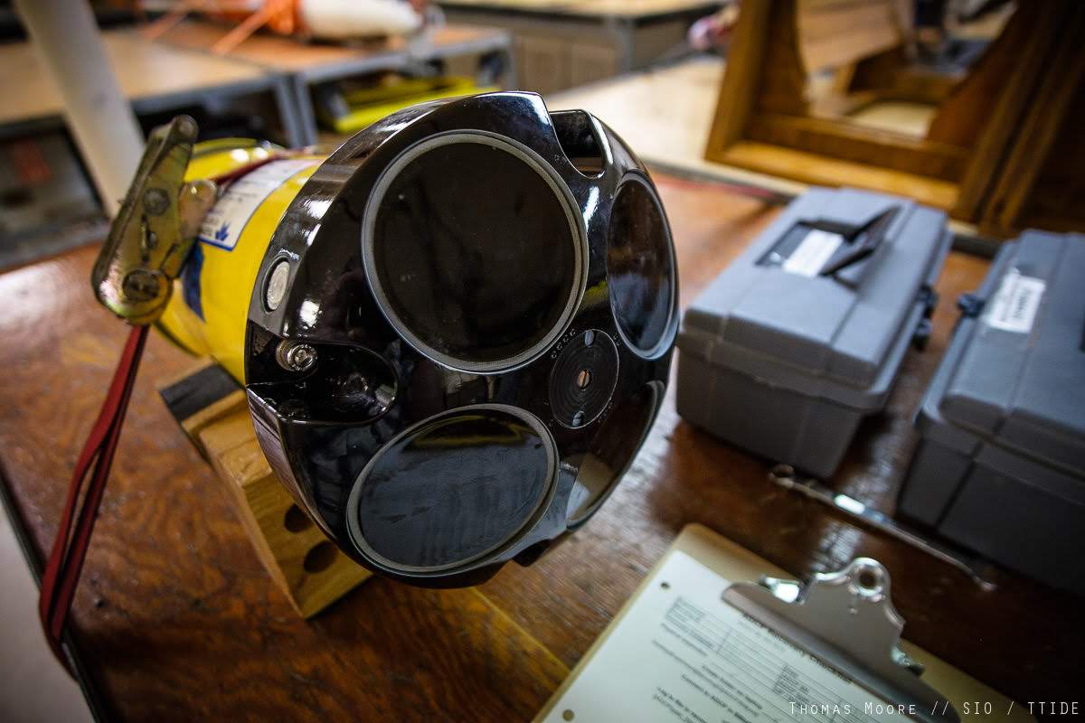
Have you ever wondered what sampling scheme to use when setting up your ADCP? The instrument can ping continuously at a set rate, or rapidly send a bunch of pings in burst mode. But what is better? I have asked myself this question in the past, often at sea when getting instruments ready for a mooring deployment. Here are some advantages for either mode for the next time I am out there. Maybe you find these helpful as well. Send me an email if you disagree or have any advice!

The ocean signal is usually weak enough that you need to average over a handful of pings to push the noise amplitude of your measurement below what you would like to observe. How the pings are spread out matters for the average.

Noise floor

Start with the part that does not depend on the sampling scheme at all. Inherent measurement noise is uncorrelated from ping to ping, so averaging $N$ pings reduces it by $\sqrt{N}$ however the pings are distributed in time. Sixty rapid pings inside a minute and sixty pings spread over ten minutes have the same noise floor.

Sampling error

The sampling scheme decides the gap between the pings you took and the average you wanted. Call $\hat{u}$ the ensemble-average over $N$ recorded pings, and call $\bar{u}_T$ the true average of the flow over the same ensemble interval $T$, the number you were after. The $N$ pings sit inside a window $W$. Burst sampling has $W = \tau$, the burst length. Continuous pinging has $W = T$. The variance of the miss, $\mathrm{Var}(\hat{u} - \bar{u}_T)$, consists of two terms:

with $\sigma_p$ the single-ping noise, and $\sigma_s$ and $T_\mathrm{int}$ the amplitude and integral timescale of the motions you are averaging over, which you never meant to resolve. Neither scheme biases the mean, so that variance is also the mean square error of one ensemble, and its square root is the error bar you would put on a single point of the record.

The first term counts pings. The second counts independent samples, $N_\mathrm{eff} = W/(2 T_\mathrm{int})$, and the length of the sampling window sets that number. The ping count does not enter. This is the standard effective-degrees-of-freedom result (see for example Thomson and Emery’s Data Analysis Methods in Physical Oceanography).

A one-minute burst every ten minutes samples over $W = 1$ min where continuous pinging samples over $W = 10$ min, so the burst ensemble carries ten times the sampling-error variance, roughly three times the standard error, at more or less the same power consumption.

The same cost shows up in a spectrum, as aliasing. Motions with periods between the burst length and the ensemble interval are too slow for one burst to average away and too fast for the record to resolve, so every burst catches them at a different phase and that scatter folds down into the band you were trying to measure. Nothing downstream separates it from real signal again. Pinging across the whole interval averages those motions away before they reach the record. For tides or internal waves under an energetic high-frequency band, that is reason enough on its own to ping continuously.

Burst length against decorrelation time

The ratio $\tau/T_\mathrm{int}$ carries the whole comparison, and the case for burst mode turns out to be the same equation read at the other end. At $\tau \gg T_\mathrm{int}$ the burst behaves like continuous pinging with fewer degrees of freedom, which is the cost above. At $\tau \ll T_\mathrm{int}$ every ping in the burst sees one realization of the flow, $N_\mathrm{eff}$ falls to one, and the burst average becomes the instantaneous velocity plus $\sigma_p/\sqrt{N}$.

So a burst-average is a very good quasi-instantaneous velocity measurement. The property that costs you accuracy on the mean is the same property you are paying for when you want the snapshot.

Reasons to pick burst

• Vertical velocity. Burst snapshots pay off most for vertical velocity. The noise geometry here is often read backwards: for a Janus pair at beam angle $\theta$ from vertical, $\sigma_u/\sigma_w = \cot\theta$, about 2.8 at the usual 20°, so $w$ is the quieter component per ping. $w$ itself is smaller by two or three orders of magnitude, though, and the events that produce it are short. Of everything the instrument measures, $w$ needs the most averaging and tolerates the least of it. Burst mode is the configuration that offers both.
• Turbulence methods need it. The structure-function estimate of $\varepsilon$ ( Wiles et al. 2006, and Lucas et al. 2014 for the moored case) and the covariance method for Reynolds stress ( Lu and Lueck 1999) all rely on rapid pings resolving the turbulent band. For a long deployment this is only possible with burst sampling.
• You can measure your own noise floor. Rapid pings inside a burst let you estimate $\sigma_p$ from the high-frequency plateau of the within-burst spectrum, or from differences between adjacent pings, without taking the manufacturer’s number on faith.
• Power. I am not sure if this actually saves much battery on commercial ADCPs. The instrument could sleep between bursts while continuous pinging keeps it awake, which may increase endurance compared to continuous pinging where the instrument goes to sleep between each ping. The instrument’s planning software may help quantifying this.
• Scheduling. On a mooring carrying several acoustic instruments, bursts can be interleaved so instruments stay out of each other’s way.

Reasons to pick continuous

• Better averages. Discussed above. This often tips the scale for continuous sampling.
• Extremes. A burst is as likely to land inside an event as outside one, so the mean survives a low duty cycle. Maxima do not. The largest velocity in a tenth of the record is smaller than the largest in all of it, and a nonlinear wave that lasts two minutes is either caught in a burst or invisible. Quote a maximum from burst data and you are describing your sampling scheme as much as the flow.
• Recoverability. Continuous pinging costs you the snapshot and some battery. Burst mode costs you a decision about $\tau$ against $T_\mathrm{int}$ that you had to make before you knew what $T_\mathrm{int}$ was, which you cannot revisit at a later time in the office.

Timing between pings

The $\sqrt{N}$ scaling assumes ping errors are independent. Ping faster than the scattering volume decorrelates and successive pings sample a partly correlated scatterer field, which will cost some of that $\sqrt{N}$. I am not sure how large the effect is.

Reverberation may matter for the burst ping interval. Pinging again before the previous ping’s echoes have faded and the new profile lands on top of them. The instrument already enforces a minimum interval covering its own profiling range, so the case to watch is a strong reflector outside that range, the surface for an uplooker or the bottom for a downlooker, returning after the profiling window has closed. How much margin this needs depends on geometry and frequency.

Continuous pinging by default

Continuous pinging is my default unless there are good reasons for bursts. Turbulence estimates would be a reason. A regime where the vertical velocity is expected large enough to be measurable at all could be another. Outside of those, spreading the pings evenly leaves the averaging decision for later once I can look at the signal. Picking the averaging scheme later only works if single pings are recorded (no ensemble averaging in the setup). I usually record every ping.

Whatever you end up picking, you’ll probably end up with a dataset full of mysteries. At least that’s what usually happens to me. Also: velosearaptor is ready to handle either sampling scheme.